Motion Control Programming Course: Servo and Stepper System Integration

2025-11-25 14:50:09

Modern motion systems no longer live in isolation from the power room. When you hang multiple servo axes and high‑inertia stepper drives on an industrial UPS or inverter bus, every programming decision you make shows up in bus loading, voltage sag behavior, and overall plant reliability. That is why a serious motion control programming course must teach servo and stepper integration from both the control and the power‑system side.

What follows is a structured guide to the core concepts and programming practices I emphasize when training engineers on servo and stepper integration, drawing on work with packaging, CNC, material handling, and process lines backed by industrial UPS and power protection systems. The content is grounded in guidance from vendors such as Anaheim Automation, AutomationDirect, Control.com, Omron, Galil, Parker, and PMD Corp, and built around problems you actually see on a live machine, not just in a textbook.

Why Integrating Servos and Steppers Matters

In real plants, you rarely get a “pure” motion technology. A packaging cell might use a high‑performance servo on a flying shear axis, economical steppers on change‑over mechanisms, and simple induction motors with VFDs for fans and pumps. AutomationDirect’s motion control guidance highlights this spectrum clearly: steppers and servos together provide the “muscle,” while PLCs and drives provide the “brain and nerves.”

Servos excel where you need precise, smooth motion over a wide speed range and the ability to hold position at zero speed. Anaheim Automation’s servo motor material lists robotics, CNC machine tools, packaging lines, labeling, diagnostics, and automated guided vehicles as typical servo domains. Stepper systems, by contrast, shine in cost‑sensitive but still fairly precise positioning jobs such as cut‑to‑length rigs, indexing tables, and small XY stages, as described in AutomationDirect’s Motion Control Explained and Contec’s motion control basics.

From a power perspective, both technologies draw their energy from the same UPS‑backed or inverter‑fed distribution. Servos with high peak torque capability push large but brief current spikes into your power system during acceleration. Steppers tend to pull more constant current at lower speeds and can run hot if misapplied. When you integrate both under one controller and one power bus, you must understand how programming choices—trajectory shape, homing strategy, indexing patterns—affect electrical stress, not just mechanical performance.

Foundation: From Servomechanism Theory to Modern Drives

What a Servomechanism Really Is

Several of the better vendor guides start from the same point: a servo is not a specific motor type; it is a closed‑loop control concept. Anaheim Automation defines a servomechanism as an automatic device that uses feedback and error‑correction to control motion, whether that motion is an electric motor, a hydraulic actuator, or a furnace temperature.

A servo motor in that context is any DC, AC, or brushless DC motor used inside a closed‑loop system with a feedback device—typically an encoder or resolver. The controller issues target position, speed, or torque, the feedback device reports the actual value, and the controller drives the difference toward zero through one or more control loops. Omron’s servo basics and Monolithic Power’s servo technology overview both reinforce this architecture: controller, drive, motor, feedback, and mechanics, with nested loops for current, speed, and position.

Historically, this idea goes back to mechanical steam‑engine governors and the “servomoteur” terminology coined in the 1800s for ship steering systems. Today, the same principle plays out in compact, DSP‑based drives on your machine floor.

Servo vs Stepper vs Simple VFD

For a programming course, you need a clear mental model of where each technology belongs. The sources we have align quite well on this.

AutomationDirect’s and Omron’s materials differentiate three broad categories. Servo systems are closed‑loop, use feedback, and are tuned; they deliver high position and speed accuracy, fast response, and high torque at speed. Stepper systems are usually open‑loop, receive a pulse train, and step a fixed angle per pulse. They can give high positioning resolution but will not self‑correct if they miss steps. Inverter‑driven induction motors paired with a VFD are best when you only care about regulating speed or torque, not exact position. Control.com’s Allen‑Bradley servo programming article notes that for pumps and fans, a simple motor plus VFD is more appropriate than a full servo.

This course uses that division heavily when we discuss axis selection and when we decide whether an axis belongs on the UPS‑protected “critical motion” panel or the standard VFD panel in the electrical room.

Comparing Servo and Stepper at a Glance

The vendor notes support a concise comparison, summarized here.

Aspect	Stepper System (Typical)	Servo System (Typical)
Control style	Mostly open‑loop pulse train, no feedback	Closed‑loop with encoder or resolver feedback
Position behavior	Fixed step angle per pulse, can lose steps if overloaded or over‑accelerated	Actively corrects error; holds final position even under varying load
Speed range	Best at low to moderate speeds; torque drops at higher speeds	Wide speed range, including high speed and zero‑speed holding
Torque and holding	High torque at low speed and strong holding torque when energized	High torque over a broad range; uses feedback to deliver required torque
Complexity and tuning	Simple to set up; no loop tuning, but care required to avoid losing steps	Requires tuning and good feedback wiring; more parameters and diagnostics
Typical use cases	Indexing tables, cut‑to‑length, simple XY tables, low‑cost automation	Robotics, CNC, high‑speed packaging, registration, AGVs, precision conveyors

Motion Hardware Building Blocks

Motors and Feedback Devices

Contec’s motion basics and Galil’s servo controller notes describe stepping and servo motors from a programmer’s point of view.

A stepping motor rotates in discrete steps tied directly to the input pulse stream. Common step angles are 1.8°, 0.72°, and 0.36°. Because each pulse advances one step, the pulse count defines how far the axis moves and the pulse frequency defines how fast it moves. For example, Contec shows a 0.72° step motor configured so that roughly 500 pulses give one shaft revolution, and five such revolutions move a carrier by about 2.0 in, requiring about 2,500 pulses.

Stepper positioning accuracy can be very high if the motor never loses steps; Contec cites a typical stop accuracy of about ±0.05° and notes that stepper motors offer strong holding force when stopped. The weakness is that if the load is too heavy or the acceleration too aggressive, the motor will fail to keep up with the pulses, a phenomenon known as “losing steps,” and the controller will not know unless you add feedback.

Servo motors, described by Anaheim Automation, Monolithic Power, Omron, and ISA, come in AC and DC designs and almost always include an integrated encoder. They run in closed loop, measuring actual shaft position and speed and feeding that back to a controller that adjusts current accordingly. The result is high‑speed response, smooth motion from low to high speed, the ability to recover from disturbances, and much higher dynamic performance than a comparable stepper.

For feedback hardware, Anaheim details the trade‑off between resolvers and encoders. Resolvers use transformer‑like windings, contain no electronics, and tolerate high temperatures and shock, which makes them attractive in harsh environments. Encoders—whether optical or magnetic, incremental or absolute—offer higher accuracy and are easier to integrate, so they are recommended in most industrial environments unless extreme heat or longevity requirements demand a resolver. The same Anaheim material lists common encoder options such as 2,500 pulses per revolution incremental encoders and 16–20 bit absolute encoders in single‑turn and multi‑turn versions.

Galil and PMD Corp describe dual‑encoder strategies for high‑precision systems, where one encoder sits on the motor shaft and a second encoder sits at the load. This dual‑loop configuration lets the drive stabilize the motor while the outer loop eliminates position error at the load, particularly useful when you have gearboxes or belts between motor and mechanism.

Drives, Controllers, and Industrial Networks

Every motion system in the notes follows the same three‑block structure that AutomationDirect explains succinctly: controller, drive, and motor. Contec’s motion control boards, Galil controllers, and PLC‑based systems from AutomationDirect and Allen‑Bradley all follow that pattern.

The controller or PLC performs trajectory generation and motion logic. It decides where and how each axis should move. The drive or amplifier converts low‑power control commands into high‑power current for the motor. The motor, fitted with feedback, generates the torque and speed to move the load.

There are two dominant command styles that the course emphasizes.

First, pulse‑and‑direction or similar step interfaces. AutomationDirect’s Motion Control Explained and Contec’s board documentation describe “step and direction,” “clockwise/counterclockwise,” and quadrature‑like schemes using OUT and DIR signals with a phase offset. In these schemes, the controller or motion board generates a high‑speed pulse train, while the drive handles current regulation and sometimes basic profiles. This approach is common for both steppers and servo drives that accept pulse inputs.

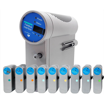
Second, networked command schemes. Anaheim’s Kinco servo drives support CAN bus and Modbus over RS‑485, allowing up to thirty‑one drives on a single RS‑485 network with cabling up to roughly 4,000 feet. Fieldbus and EtherCAT interfaces are available for tighter PLC integration. AutomationDirect’s servo and motion articles describe drive‑level indexing drives that store multiple motion profiles and are commanded by a PLC via Modbus TCP or hardwired I/O. ISA’s servo motion basics emphasize that modern servo drives frequently live on industrial Ethernet networks such as EtherCAT, PROFINET, EtherNet/IP, and similar protocols.

When you integrate these drives on a UPS‑backed bus, you must consider not only normal running current but also peak overload current. Anaheim notes that Kinco servo drives can supply up to about three times rated power for short periods to handle overloads. Programming sharp acceleration ramps on many axes at once may therefore pull several times the nominal current from your UPS or inverter, something we explicitly model in the power‑system segment of the course.

Programming Servo Axes: Concepts You Will Practice

Scaling Mechanics into Engineering Units

Control.com’s servo programming example with Allen‑Bradley and a Festo ball screw actuator illustrates a point that confuses many beginners: if your motion code says “move 6.0,” what does that mean physically?

In the example, a gearbox with an input‑to‑output ratio of 1:5 drives a ball screw with a pitch of about 0.14 in per revolution. The controller must know both the gearbox ratio and the screw pitch so it can convert encoder counts to inches or another engineering unit. AutomationDirect makes the same point for pulse/direction systems: your pulse frequency must stay within the capabilities of the PLC output module and the drive, and your resolution must be set so the axis can achieve both the top speed and the positional granularity you need.

In the course labs, you learn to calculate and configure these mechanical ratios so that a command like “move to 12.0” actually moves the slide about 12 in, and you verify it at the machine with a dial indicator or tape measure, not just in software.

Homing and Referencing Strategies

Before you can use absolute moves, the controller must agree with reality about what “zero” means. Control.com’s material emphasizes homing—also called referencing—as a critical step for servo systems that rely on incremental encoders or power‑up alignment.

Several homing strategies appear across the notes. Home‑to‑sensor methods use a mechanical or optical switch to detect an origin position. Home‑to‑torque methods move the axis until it bumps a hard mechanical stop and measure torque rise. Contec’s ORG motion functions go further and let you specify a preferred direction of approach, avoid the need for a separate “near origin” sensor by carefully controlling deceleration, and define how logic levels are interpreted. Many drives also support simply asserting the current position as zero in applications such as conveyors where absolute reference is not critical.

Absolute encoders, highlighted in AutomationDirect’s servo‑accessibility article and Anaheim’s encoder options, retain position over power cycles, reducing or eliminating the need for homing at startup. However, even in absolute systems, I recommend keeping a homing routine in your codebase to recover from mechanical work, feedback replacement, or commissioning scenarios.

Motion Types and Profiles

Most industrial drives and motion boards implement the same family of motion commands, even if the instruction names differ. Across Contec, AutomationDirect, and Control.com you see several types.

Point‑to‑point moves, sometimes called PTP, move from one position to another with defined acceleration, speed, and deceleration. Contec notes that some boards can even change the target position on the fly during acceleration or constant‑speed segments.

Jog moves run continuously at a set speed until a stop or limit input occurs. They are essential for commissioning and maintenance and are typically exposed on HMIs so technicians can jog axes forward and backward in continuous or incremental modes.

Origin or ORG moves are specialized routines for homing which, in Contec’s implementation, are executed largely in hardware once configured. That reduces the amount of custom origin logic you need to write.

On the profile side, Contec distinguishes constant‑velocity profiles, linear acceleration and deceleration profiles (sometimes called trapezoidal), and S‑curve profiles that smooth the onset of acceleration to reduce jerk. AutomationDirect’s and AutomationDirect’s servo articles echo these same profile shapes and emphasize their importance in protecting mechanics and product from sudden shocks.

For multi‑axis machines, Contec’s interpolation support shows how controllers can coordinate axes using point‑to‑point, linear, and circular interpolation. AutomationDirect and ISA describe more advanced patterns such as camming, electronic gearing, and registration, where one “master” axis defines a virtual cam or gear relationship for several follower axes.

From a power and reliability perspective, the key is that every sharp corner in a profile becomes an electrical and mechanical shock. In labs, I have students compare bus current and PLC diagnostics when running the same axis with a square‑cornered profile and with a smoother S‑curve. Even without adding external instrumentation, the difference in drive alarms and UPS loading is usually obvious.

Structuring Code and Diagnostics

Control.com’s Allen‑Bradley example lays out a programming structure that generalizes well to other platforms. The servo axis logic lives in dedicated routines, separate from the main sequence logic. Setup routines handle enabling the drive after safety interlocks are satisfied, assigning parameters, and dealing with faults. Motion routines handle issuing moves and checking that the axis actually starts and completes them.

A common pattern they show uses a user‑defined data type to hold move parameters, then an array where each element is a “teachable” position. The sequence code simply selects an index and copies that structure into a single motion instruction such as a move‑absolute block. HMI screens then let maintenance staff jog an axis into position and push the current axis value back into a selected array index.

On diagnostics, both Control.com and Contec stress surfacing both drive‑level alarms and application‑level conditions. Drives report faults such as overcurrent or overtemperature using codes that you look up in manuals. Applications add conditions like “not in position,” “tooling not clear,” or “command did not complete.” Contec’s motion boards include dedicated inputs and outputs for alarm signals, deviation counter clear, and event outputs when counters hit programmed values, letting hardware logic react quickly to fault conditions while the PLC or PC logs and displays details.

From a reliability‑advisory standpoint, I insist that course projects log any motion fault with axis name, commanded move, drive code, and any relevant power‑system context such as UPS remaining ride‑through where that data is available from the UPS network card.

Programming Stepper Axes and Hybrid Systems

The motion‑control basics from Contec and AutomationDirect show that programming steppers is not fundamentally different from programming servos, but you must think in terms of pulses and open‑loop behavior.

A stepper axis typically receives pulse trains from a PLC high‑speed output or a motion control board. AutomationDirect cites low‑cost PLCs with pulse outputs in the tens or hundreds of kilohertz, with newer modules reaching about 1 MHz. Contec’s boards can generate pulses based on target distance, speed, acceleration, and deceleration while also monitoring limit and origin sensors.

The same high‑level motion concepts exist: point‑to‑point moves, jog moves, and origin moves. Interpolation and multi‑axis synchronization are available as well. Contec demonstrates multi‑axis synchronized start and stop across multiple boards, with up to sixteen boards controlling as many as one hundred twenty‑eight axes, and with on‑board memory that can switch between motion frames in about one microsecond. That is powerful for building complex profiling without loading the host CPU, but it also means your motion subsystem can draw sudden bursts of current very quickly.

Because standard steppers are open‑loop, the burden is on you to choose accelerations and loads that do not cause losing steps. The Contec material explains losing steps as a failure of the motor to keep up with rapid changes in pulse frequency or excessive load torque. In the course, I pair this with PMD Corp’s discussion of servo tracking error to show that an “invisible” open‑loop error on a stepper can be thought of as a saturated servo loop with no feedback. Both cause mechanical and process issues; one is just harder to detect.

Hybrid architectures that mix steppers and servos are common in AutomationDirect’s Motion Control for the Many guide. Basic axes might use steppers with indexing drives, while high‑performance axes use servo drives with fieldbus connections and built‑in motion logic. Standard PLCs or micro‑PLCs coordinate everything. As a programmer, you must abstract axis types so that higher‑level logic only sees “axis moves,” not the difference between a pulse train and a fieldbus command.

Advanced Topics: Tuning, Feedforward, and Troubleshooting

Once a basic system is running, the difference between an acceptable machine and a robust one comes from how you handle tracking error, noise, and low‑speed behavior. PMD Corp’s “Common Motion Problems and How to Fix Them” and their servo noise article provide a structured way to tackle these issues.

Reducing Tracking Error with Feedforward and Better Loop Structures

PMD Corp explains that position tracking error is the gap between commanded and actual position during motion, not just at the final stop. In machine tools, glue and sealant application, plotting, and guidance, this dynamic error matters a great deal.

Acceleration feedforward is one of the most effective tools available. The idea is to pre‑apply a motor command proportional to the commanded acceleration, anticipating the torque needed to accelerate the load. When load inertia is reasonably well known and stable, this can substantially reduce tracking error without cranking proportional gains to the edge of instability.

Velocity feedforward works similarly but targets friction and back‑EMF effects. It applies a command proportional to commanded speed, which is especially useful when an amplifier operates in voltage mode without an inner current loop.

When simple position‑only PID loops reach their limits, PMD Corp and Galil both suggest cascaded position and velocity loops. In this structure, an inner velocity loop controls speed using either differentiated position feedback or a dedicated velocity estimate, while an outer position loop commands velocity targets. PMD discusses specialized velocity estimation such as 1/T circuits that measure the time between encoder edges, and digital filters that reconstruct velocity from granular position feedback. These are advanced topics in the course, but they show students how control structure choices influence both performance and power draw.

Smart Sampling and Filtering

The same PMD guidance warns against blindly increasing servo loop rates. The mechanical time constant of the axis should be much larger than the sample period; otherwise you inject high‑frequency noise that does more harm than good. Sometimes slightly slowing the loop or adjusting the derivative sampling period results in smoother motion and lower noise without sacrificing accuracy.

Filtering tools are essential here. PMD describes biquad filters that act as low‑pass, band‑pass, or notch filters tuned to mechanical resonance frequencies discovered via sinusoidal sweeps. AutomationDirect and Omron mention similar software oscilloscope and tuning features in modern drives. In the course lab, we use a drive’s built‑in scope to compare commanded and actual motion while adjusting filters, and we look at how excessive filtering can trade off responsiveness for stability.

Handling Low‑Speed Jitter and Noise

Two recurring problems in servo courses are noisy holding behavior and rough motion at very low speed.

PMD’s servo motor noise article points to derivative gain as a frequent culprit. Excessive derivative gain amplifies high‑frequency encoder noise and turns the motor into a loud, vibrating “speaker.” Reducing derivative gain or using different gain sets for motion and holding can dramatically quiet an axis. They also note that current‑loop tuning and PWM frequency matter. For example, low‑inductance motors may require higher PWM switching frequencies than older, larger motors to reduce current ripple and related acoustic noise, though any such change must be balanced against switching losses in the drive.

For low‑speed smoothness, PMD’s common problems article explains that digital encoders provide position in discrete counts, so as speed drops, motion can appear “bumpy.” Remedies include using higher‑resolution encoders, reducing sample rate to average over longer intervals, using dedicated 1/T velocity estimation, or even adding analog tachometers where vendor hardware supports them. In some niche applications like barcode scanners, they mention phase‑locked loop controllers for extremely constant speed, though those are less flexible for variable‑speed motion.

Mechanically, the same article reinforces a theme echoed by Servo System Application Tips and Kollmorgen’s servo elements: your servo is only as good as your mechanics. Couplings, gears, bearings, slides, and cables introduce friction variation and compliance. Direct‑drive arrangements reduce these issues, but even there you can see friction changes along a track due to ball bearing circulation or imperfect rails. The course spends significant hands‑on time teaching students to separate mechanical problems from tuning problems so they do not “over‑tune” a fundamentally bad mechanism.

Power, Reliability, and Motion: Designing for UPS and Inverter Systems

Although none of the vendor articles we have focus specifically on UPSs, reading them as a power‑system specialist makes a few priorities obvious.

First, overload capability and motion profile choices interact directly with power margins. Anaheim notes that Kinco servo drives can deliver up to about three times rated power for short overload events. If you design motion schedules that accelerate several large axes simultaneously on a UPS‑backed panel, those peaks can stack and stress both the drives and the UPS inverter. In the course, I encourage staggering high‑torque events in software when power margins are tight, especially on retrofit lines where the UPS cannot easily be upsized.

Second, regenerative energy and braking must be considered. Several servo guides reference dynamic performance and rapid deceleration without explicitly talking about where that energy goes. On a typical system, that energy either charges the DC bus, is burned off in braking resistors, or, in some configurations, is pushed back toward the AC supply. From a reliability perspective, you want braking and bus‑sharing strategies that keep bus voltage within drive limits even when a UPS is feeding the system. That may mean coordinated deceleration profiles and conservative braking resistor sizing.

Third, disturbance ride‑through matters. ISA’s servo basics and AutomationDirect’s PLC‑based motion articles both point out that servo drives are intelligent, microprocessor‑based devices with rich diagnostics. In a power event, those diagnostics are only useful if the drives stay powered long enough to log meaningful data. For critical axes, I recommend designing both the UPS capacity and the motion control “safe stop” sequences so that regenerative and transient events do not cause nuisance trips. That often means integrating drive fault bits into higher‑level logic and practicing simulated power disturbances during commissioning.

Finally, grounding, shielding, and wiring are not only EMC topics; they are reliability topics. Omron’s and Parker’s servo guidelines emphasize proper separation of power and signal cables and the use of shielded twisted pair for sensitive feedback lines. Contec’s encoder and I/O descriptions assume clean signals. In plants with noisy power or long cable runs, I have seen encoders miscount or drives misinterpret I/O due to poor reference bonding between UPS outputs, drive chassis, and control cabinets. For that reason, the course devotes a segment to power‑system grounding and bonding strategies that respect both electrical code and motion‑control signal integrity.

Designing Your Learning Path Through the Course

A motion control programming course that truly prepares you for real plants needs to do more than walk through datasheets. Based on the combined guidance from Anaheim Automation, AutomationDirect, Control.com, Contec, Omron, Galil, ISA, Parker, PMD Corp, and others, I structure the learning path in four broad phases.

You start with fundamentals: definitions of servomechanisms, open‑ versus closed‑loop control, and the role of feedback, along with servo versus stepper versus VFD trade‑offs. You then move into hardware awareness, learning how controllers, drives, motors, encoders, I/O, and networks fit together, and how mechanical elements such as screws, belts, and gearboxes define your scaling and performance limits.

The third phase centers on programming patterns. Here you work through real servo and stepper examples: scaling mechanics to engineering units, implementing homing routines, building jog and point‑to‑point motion, organizing code into reusable routines, and linking everything to HMIs for jogging and teaching positions. You learn to use drive software tools such as oscilloscope views, alarm histories, and auto‑tuning features, as described in vendor tools like Anaheim’s Servo+ and various PLC motion packages.

The final phase is reliability‑focused. You learn feedforward and advanced loop structures for better tracking, use filters and sample‑time adjustments to fight noise and resonance, and practice diagnosing low‑speed jitter, excessive noise, and tracking errors using the approaches laid out by PMD Corp and others. Crucially, you overlay that with power and UPS considerations so your motion code is friendly to the electrical infrastructure it lives on.

By the end of that path, you can look at a mixed servo and stepper installation on a UPS‑backed bus and reason confidently from power room to PLC ladder to encoder count.

Quick FAQ

Do I always need a dedicated motion controller, or is a PLC with motion instructions enough?

AutomationDirect’s motion articles and ISA’s servo basics show many successful systems built both ways. For simple or moderate systems, a PLC with built‑in high‑speed outputs or motion modules can control a few axes very effectively, especially when paired with drives that include indexing and basic profiles. For higher axis counts, tighter synchronization, or more advanced profiles such as complex camming and registration, a dedicated motion controller or a PLC platform with motion‑optimized networks such as EtherCAT becomes more appropriate. In practice, the decision often comes down to how many axes you have, how tightly coordinated they must be, and how much reuse you want across machines.

Can I safely mix vendors for PLCs, drives, and motors?

ISA’s guidance notes that it is possible to mix vendors, but also that using an integrated motion portfolio from a single supplier simplifies engineering and support. Servo System Application Tips cites user preference for matched drive‑motor sets from one vendor to reduce wiring and configuration problems. In my experience, if you mix vendors you should budget extra time for network configuration, feedback compatibility checks, and support coordination when something goes wrong. On UPS‑backed systems, I also pay close attention to how each vendor handles overload, regenerative energy, and ride‑through so that combined behavior does not surprise the power system.

When is a stepper a better choice than a servo in an industrial UPS‑backed system?

AutomationDirect and Contec both make the case that steppers are still the best option when you need reasonably precise positioning at low to moderate speeds, with modest dynamics, and you want to keep cost and complexity down. Typical examples are indexing tables, small XY stages, and simple cut‑to‑length mechanisms. On a UPS‑backed bus, steppers can be attractive because their current draw is more predictable and you avoid the additional tuning and feedback wiring effort. When your application demands high‑speed motion, tight tracking during motion, and quick recovery from disturbances, the additional complexity of a servo system usually pays off.

For engineers working in facilities with serious expectations around uptime and power quality, learning to program and integrate servo and stepper systems is no longer optional. It is the bridge between the motion diagrams in your design review and the UPS load profiles and reliability metrics that define whether your line keeps running when the power system is under stress.